Animal inspired robotics. An interactive simulation for BIOE97156

This is meant to be an auxiliary short explanation and discussion about target interception for Imperial College’s module on Animal Locomotion and Bioinspired Robotics (ALBiR).

Part 1: Simulation of target interception

For the simulation seen below, the robot is initially positioned as specified in the coursework. Hitting the “Play” button will start the simulation with default settings. These are: robot and prey position as per specification on coursework (120cm away from each other), robot speed is 100cm/s, prey speed is 70cm/s, the robot’s controller only has PI gain and the prey follows a straight path. However, there are also buttons on the side that allow for the modification of the simulation, these are:

• Play: Start the timer and simulation
• Fixed Init: If active the robot and prey will be positioned as per specification in the coursework
  • When deactivated, the user can place the robot, prey and obstacle in a position of their liking
• Reset: Stop the simulation and timer and set simulation back to the original state
• C. Bearing: Activate the constant bearing pursuit (+15deg)
• Proportional: When activated the robot controller only has D gain
• Fast prey: When activated increases the prey speed from 70cm/s to 100cm/s
• Sinusoidal prey: Prey follows a sinusoidal path instead of straight line

The Effect of different variables in time-to-capture:

The simulation seen here is quite flexible and allows us to generate different scenarios on the go. Playing the simulation as it starts by default is one of the most naive implementations of the algorithm, with the slower prey the time-to-capture (TTC) is 1.43s and when the robot is set to the fast setting the TTC is 3.09. However, if a constant bearing is applied, the TTC are significantly reduced, especially the one with the faster prey, which are now 1.03s and 1.43s respectively.

The effect of the sinusoidal path is harder to measure as it depends greatly on the starting position of the robot, the reader is therefore encouraged to tinker around with the initial conditions by deactivating the “Fixed init” and observing the results. However, here again the constant bearing can massively improve the TTC, to the point that if set to the fastest settings, without the constant bearing the robot may not be fast enough to catch the moving target.

Activating the proportional option makes the controller have only a differential gain as per the coursework specification. The author was unable to set a value for the differential gain that would generate optimal results on its own, however the combination of both proportional and differential gain in a PD controller could improve performance. In the real-life implementation, the robot does have a differential gain in its controllers which improves the behaviour and TTC, especially in the sinusoidal path, as the robot is able to “predict” where the prey is moving.

Finally, initial conditions obviously play a major role in the TTC, but it also shows the robustness of the current implementation. The robot will be able to catch the prey in most scenarios and can deal with the obstacle in an elegant manner without majorly disrupting the time to capture.

Sensorimotor delay

Sensorimotor delay can be one of the main challenges in robotics. Real-time information is hard (rather, impossible) to have and the best we can do is try to reduce this delay. However, there are multiple ways to reduce the effect of such delay, for instance, adding a differential gain can introduce a type of “prediction” to our controller that could take care of small latencies in the sensing and/or processing. Another option would be to implement an actual prediction process by measuring the distance and angle at multiple time-points and finding their derivatives. This would provide the agent with the velocity and positions in time of the prey in polar coordinates from which cartesian coordinates could be extrapolated. With these the agent could try different approaches, from parallel navigation to (if the measurements are precise enough) prediction of the target position at longer timeframes and trying to intercept the prey that way. With biological beings the latter would most likely not succeed as often, as the prey is often aware of the predator and would change its behaviour accordingly.

Parallel navigation

As stated before, parallel navigation could be an appealing solution to not only dealing with sensorimotor delay but also improving our TTC and even deal with a prey that is aware of being chased. The implementation of parallel navigation in the simulation can be rather straight forward. Given the precise and noiseless measurements, one could find the current distance and angle and their instant time derivatives, which would provide sufficient information for parallel navigation. This could be achieved by setting the desired angle of the robot w.r.t. the prey at 90deg. In real-life (or at least with our robot implementation) this could prove much more challenging. The noise in the distance and angle estimation could make our readings for the instantaneous time-derivatives worthless and would require a moving average filter to reduce the noise that would add further delays to our readings, making the extra gain of parallel navigation potentially worthless.

Using a frame of reference, such as a distant object, the user may have better luck, but this would involve running an image processing script in the frames to find which set pixels are unchanged over a long period of time (ensuring that this set of pixels is not the prey) and then using said set of pixels as a reference. However, the prey may change its course, background may change, or the frame of reference may become suddenly obstructed. It might be easier to estimate the speed of the robot by finding the turning rate of the wheels and using a moving frame of reference set at the robot as described previously.

Assuming a more ideal world, the implementation in our robot could be the following:

1. Have the servo controller keep chasing the target. This way the target never leaves the FoV and our estimations of angle and distance are kept.

2. Store these values over time and make average time-derivatives that would denoise the signal.

3. Set the controller’s target angle to that of the estimated velocity vector of the prey

4. The speed of the agent can (and ideally should) be greater than that of the prey, thus getting closer at each timeframe.

Part 2: summary and discussion of the robot implementation

During the spring term of 2020 in ALBiR we have studied the different ways locomotion and environment perception and interaction works in the animal kingdom. From biped motion, to visual recognition and target pursuit, we have explored Nature’s solution for these problems. Copying Nature Inspired by Nature we were expected to take what we had learnt and use it to the real world. A small robot was built using two brush motors, a Raspberry Pi and a Pixy2 camera attached to a servo. Our aim is to make the robot a competent predator by implementing target tracking algorithms that work in the real world.

To make this work the robot needs to be competent in two main areas, sensing the environment and reacting accordingly.

Sensing the environment

Distance estimation

One of the most important pieces of the algorithm is a precise distance estimation function. Without it, critical information such as angles with respect to obstacles and target would be impossible to acquire. Our only input for estimating said distance is the camera feed, therefore, we are determining the distance by the angular declination below the horizon. As it can be seen from the figure below (Ooi et al. 2001), we can find the distance to the target (d) by measuring its angle with respect to the horizon.

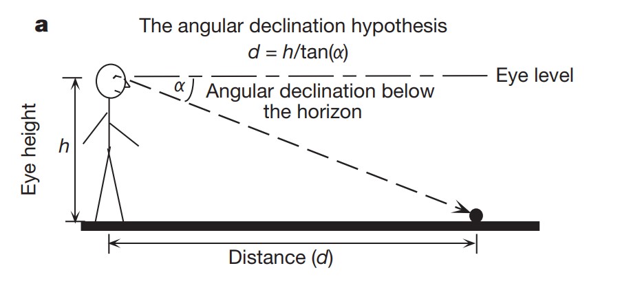
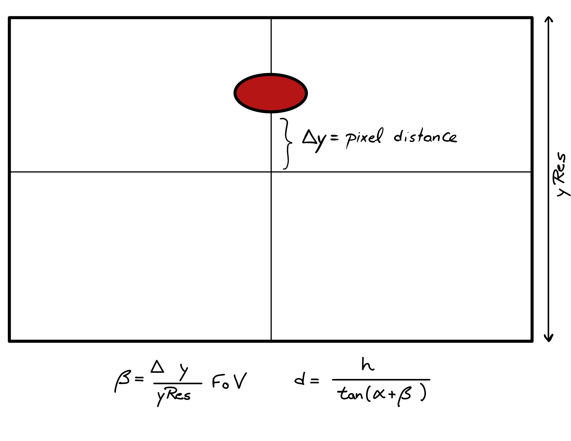
For the robot, we know the camera to be tilted by 20 degrees, which will be our initial angle (alpha). To which we would like to add another angle (beta) that will be the inferred angle within the robot’s field of view as seen below.

This process allows us to measure distances, which is required for the following steps.

Angle estimation

Similarly to the distance estimation, the angle estimation is inferred by the pixel distance to the centre of the feed and the camera’s FoV.

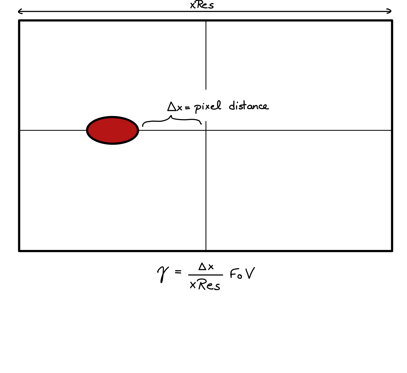The final angle will be gamma + servoPosition, the servo position is returned in angles already by the servo library in Python, therefore it is very easy to find.

The controllers

The robot requires two different controllers to work properly. The first controller manages the “head” (the servo motor attached to the camera), whereas the second controller manages the robot’s body position by setting the turning rate of the wheels to steer left or right.

The different controllers exhibit different behaviour, the head controller needs to be both smooth and fast adapting as the prey leaving the FoV would mean losing the ability to estimate both distance and angle, which would significantly handicap our robot’s ability to catch the prey. Therefore the head controller PID(0.04, 0, 0.08) has a higher pGain and dGain that can even overshoot if necessary to keep the prey in the FoV.

The wheel’s controller requires a smooth behaviour avoiding abrupt changes the PID(0.005, 0, 0.04) is slightly overdamped. This controller also helps in the obstacle avoidance, when the obstacle leaves the FoV, the robot has no way of knowing its position. This overdamped controller allows for smooth turning around the obstacle without turning into it even if the prey is close. (This behaviour is especially noticeable in the simulation and videos, so the reader is encouraged to inspect those thoroughly)

Making predictions

As stated before, the robot will be able to extract information about angle and distance only if the prey is in the FoV of the camera, but what happens when the prey is obstructed by an obstacle or the prey makes a sharp turn? In this instance we would like to make predictions based on our previously available information about the prey and obstacles. While the prey is seen, the robot will not only chase it, but also gather information about the prey’s and obstacle’s angle, distance, and how these change over time. When the prey is not in the FoV, a different script triggers that will use this previous information to guess both the prey and obstacle’s angle and distance in the next update. The script will make an average of the change in angle and size in the last 20 frames and use that to update obstacles’ and prey’s position and angle.

angle(t+1) = angle(t) + d/dt angle(t)

After this, the new predicted angle will be appended to the vector storing this information and the cycle can start again. However, this creates a problem as the predicted angle could grow infinitely. Therefore, a decaying factor for the dAngle is put in place so that it will decrease as time continues. This behaviour can be observed in the videos underneath. Without a prediction, the robot will stop when it stops seeing the prey, wasting time, one of the performance indicators for the target tracking algorithms.

Avoiding the obstacles

Obstacle avoidance is another of the main objectives of the coursework. The principle used in our implementation is rather simple, the robot is meant to follow the prey, but if the obstacle is within a certain threshold, we want to modify our trajectory to avoid bumping into it without disrupting our TTC. To avoid turning unnecessarily, the threshold depends on both the distance to the obstacle and the angle at which the obstacle is with respect to the robot. If the angle is greater than 30 degrees, it is unlikely that the robot will bump against the obstacle regardless of the proximity and if the target is further than a set threshold (d = 0.5m) the obstacle will be ignored. However, if both conditions are met, we want to ensure that the new trajectory is both smooth and the shortest possible path to the prey. To ensure smoothness, the desired angle cannot be changed abruptly once the conditions are met, it should be increased gradually by applying weights to the different “forces”. One of said forces pulls the robot towards the prey and the other pushes it away from the obstacle. The final desired angle fed into the controller is a normalised weighted sum of both forces, ensuring a smooth transition. The current implementation uses proximity and angle to the obstacle as compared to the thresholds to provide this normalised weight. To find the shortest path, the agent must decide whether to avoid the obstacle from the left or the right. One possibility would be to steer to the left if the object is to the right of the robot and vice versa. However, in that situation the agent is not taking into account the prey’s velocity, which can lead to problems. In the situation below, which path should the robot take?

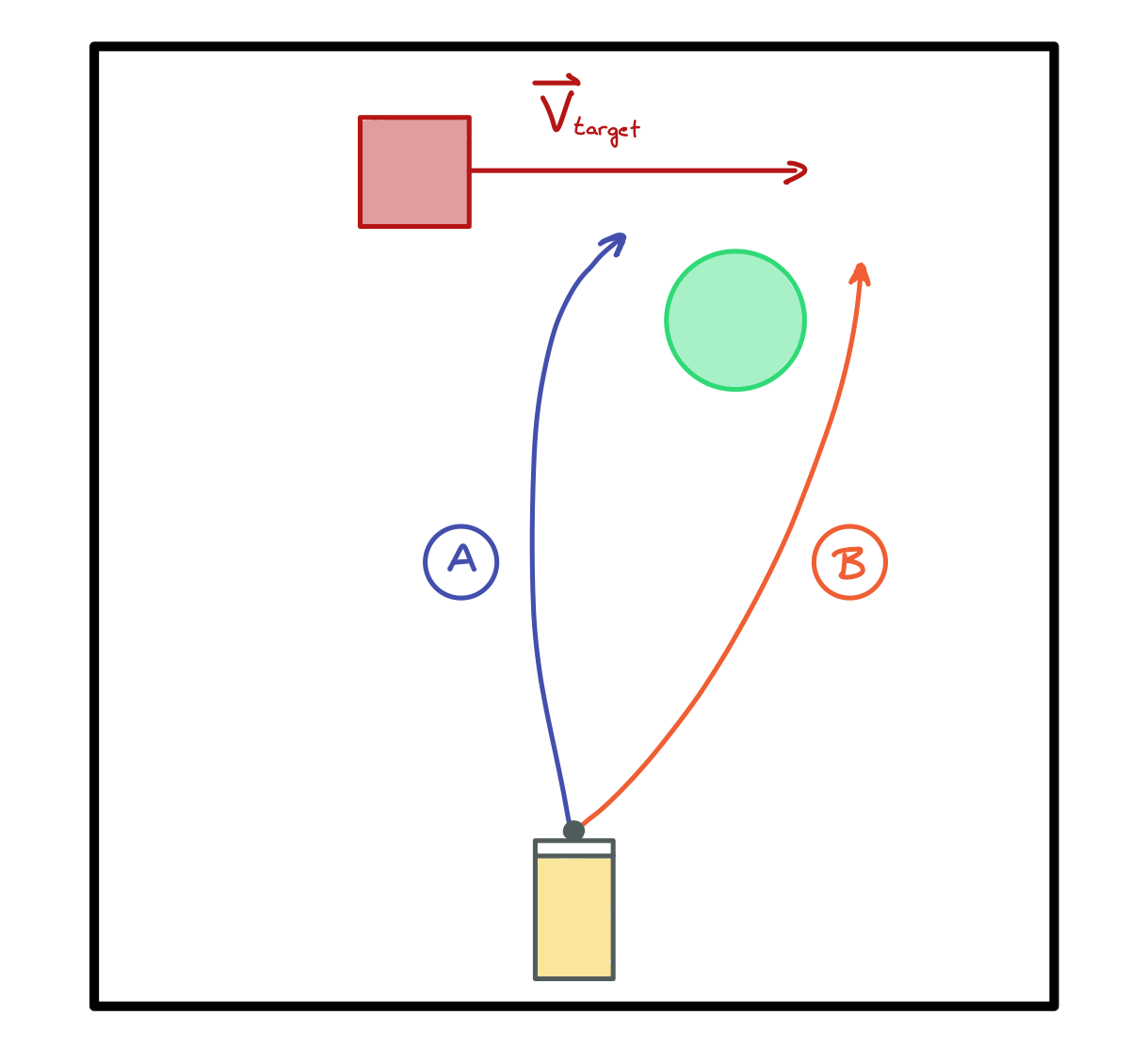
To assess this, the robot implements a small check that will take into account the prey’s velocity and proximity to the target and then the agent will choose the path (left or right) accordingly. Finally, once the path is chosen the robot also takes into account the obstacle’s width and measures the angle not from the centre but the obstacle’s side (left or right accordingly) making the maneuvering as precise as possible. In the video underneath, the robot can be seen turning right to avoid the obstacle even though the prey is on the left of said obstacle and maneuvering by narrow margin.

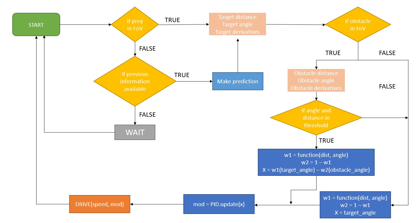
Flowchart of the implementation

Underneath a simplified flowchart can be observed that describes the robot’s behaviour, again for simplicity and to avoid redundancy, some steps previously described in detail (such as the obstacle avoidance) are greatly simplified.

Failure modes

The current implementation is pretty robust and is a slightly more complex version of the simulation shown in the website and the author encourages the reader to test the robustness of the algorithm there. However, there are several ways that still cause some problems in the real life implementation. The main source of error most likely comes from the camera, as it is very sensitive to lighting condition. A further improvement could be replacing the camera or simply implementing a more robust recognition algorithm that will also take into account the prey’s and obstacles’ shape (not only colour) to discern between false positives and adapt the brightness of the camera to detect them properly. This is a major source of concern as previously stated, the rest of the algorithm relies on reliable and accurate readings of the environment. Finally, the prediction algorithm is not perfect and any red marking could trigger a great change in angle that would therefore translate in a great derivative value that would trick the prediction algorithm into searching the target in the wrong place.

Further developments

No project is ever finished and this is no exception, even though the current implementation is quite robust, the failure modes described previously could be avoided by spending more time in the development of the agent. Additionally, I would like to have implemented an adaptive bearing. Modifying the constant bearing approach to have a greater displacement angle when the prey is changing angle quickly.